Combining Machine Learning and Logical Reasoning

(Press ? for help, n and p for next and previous slide)

Department of Computing, Imperial College London
Dec 28th, 2020

Abstract:

Perception and reasoning are two representative abilities of intelligence that are integrated seamlessly during human problem-solving processes. In the area of artificial intelligence (AI), the two abilities are usually realised by machine learning and logic programming, respectively. However, the two categories of techniques were developed separately throughout most of the history of AI. In this talk, I will introduce our recent progress on Abductive Learning (ABL), a novel machine learning framework targeted at unifying the two AI paradigms. In ABL, a machine learning model learns to perceive primitive logic facts from data, while logical reasoning can exploit symbolic domain knowledge and correct the wrongly perceived facts for improving the machine learning models. Moreover, I will present the abductive Meta-Interpretive Learning (Meta_Abd ) approach, which unites abduction and induction to learn machine learning and first-order logic theories simultaneously. To the best of our knowledge, Meta_Abd is the first system that can jointly learn neural networks and recursive first-order logic theories with predicate invention. In experiments and an application on real data, we demonstrate that ABL not only outperforms the compared end-to-end deep learning models in predictive accuracy and data efficiency, but also learns interpretable symbolic models that can be reused as background knowledge in subsequent learning tasks.

Two AI Paradigms

Data-Driven AI

Adding data to improve the model:

Image Net (1.2M images)

GPT-3 (4.5TB text)

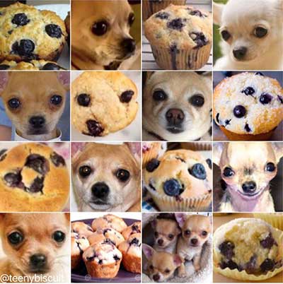
Knowledge-Driven AI

Adding knowledge to speed-up problem solving and learning:

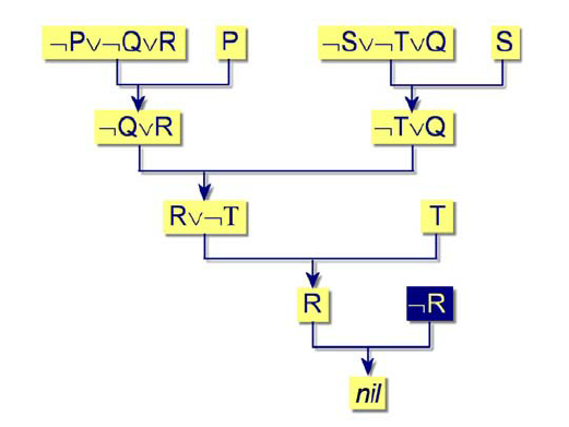
Theorem provers
Rule-based expert systems
Intelligent forms of search (semantic web, knowledge graph, etc.)
Constraint-based approaches (SAT, CLP, SMT, etc.)
Program synthesis / Inductive Logic Programming

Example: Learning Quick Sort

Examples: Background Knowledge (Primitive Predicates): Leanred Hypothesis:

Popper (Cropper & Morel, 2020)

Combining Subsymbolic and Symbolic AI

Yoshua Bengio: From System 1 Deep Learning to System 2 Deep Learning.

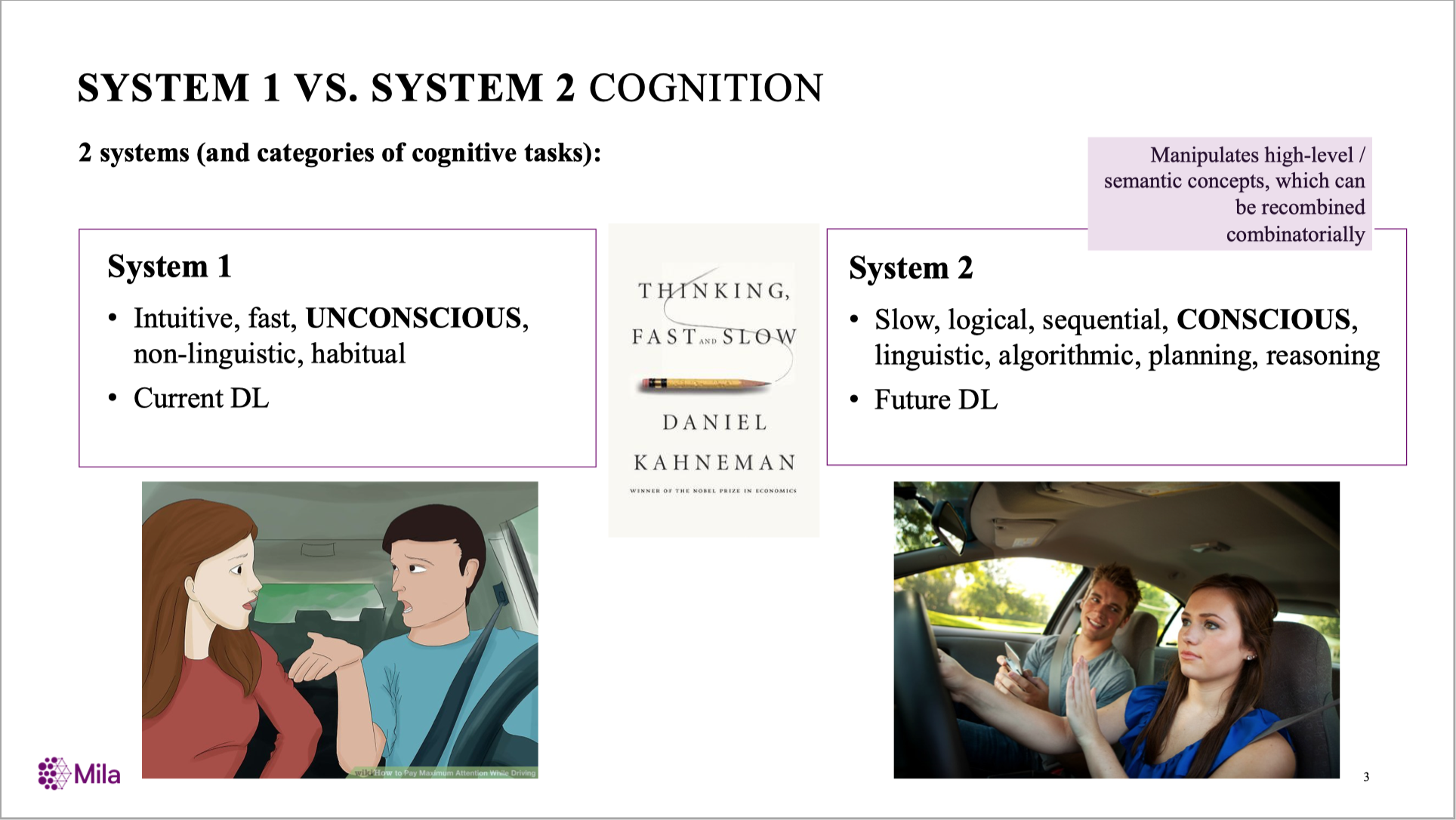
(NeurIPS’2019 Keynote)

System 1 vs System 2

Representation	Statistical / Neural	Symbolic
Examples	Many	Few
Data	Tables	Programs / Logic programs
Hypotheses	Propositional/functions	First/higher-order relations
Learning	Parameter optimisation	Combinatorial search
Explainability	Difficult	Possible
Knowledge transfer	Difficult	Easy

Why is the combination so hard?

Boolean Algebra

A Boolean algebra is a complemented lattice with binary operators $\wedge$, $\vee$ and a unary operator $\neg$ and elements $1$ and $0$ s.t. commutative, associative and distributive laws hold.

conjunction: $x\wedge y= \mathrm{inf}\{x,y\}$
disjunction: $x\vee y=\mathrm{sup}\{x,y\}$
negation: $\neg x=\bar{x}$
implication: $x\rightarrow y=\neg x\vee y$

Many-Valued Logic

Finite set $W_m=\{\frac{k}{m-1}\mid 0\leq k\leq m-1\}$ or infinite set $W_\infty =[0,1]$

conjunction: $x\wedge y=\mathrm{min}\{x,y\}$
- Łukasiewicz: $x\& y=\mathrm{max}\{0,x+y-1\}$ (“weak and”)
- Independent fuzzy set: $x\wedge y=x\cdot y$
disjunction: $x\vee y=\mathrm{max}\{x,y\}$
- Noisy-or: $x\vee y= 1-x\cdot y$
negation: $\neg x=1-x$
implication: $x\rightarrow y=?$
1. Łukasiewicz: $\mathrm{min}\{1, 1-u+v\}$
2. Gödel: $1$ if $x\leq y$ else $0$
3. T-norm: $x\rightarrow_T y=\mathrm{sup}\{z∣T(x,z)\leq y\}$
4. …

“Next-Gen” AI

Statistical relational models
- 1992: Knowledge Base Model Construction (Wellman, Breese & Goldman)
Neural relational models
- 1994: KBANN (Towell & Shavlik), PCMLP (Hölldobler & Kalinke)
- 1999: C-IL²P (Garcez & Zaverucha)
Probabilistic logic programming
- Probabilistic logic (Nilsson, 1986), Probabilistic logic programs (Dantsin, 1992)
- 1995: Distribution semantics (Sato)

Route 1:
Statistical / Neural Relational Models

Knowledge Base Model Construction

Semantics: Logical relations $\Leftrightarrow$ Statistical correlation. e.g.,

\begin{equation} A\leftarrow B_1 \wedge B_2 \wedge \ldots\wedge B_n \end{equation}

can be interpreted as:

\begin{equation} P(A,B_1, B_2, \ldots, B_n)=P(A|B_1, B_2, \ldots, B_n) P(B_1, B_2, \ldots, B_n). \end{equation}

Or, more generally, add representation learning

\begin{equation} P(A)=f(\varphi(A),\varphi(B_1), \varphi(B_2), \ldots, \varphi(B_n); \theta), \text{ where } B_i \text{ are Markov blanket of } A \end{equation}

KBANN (Towell & Shavlik, 1994)

\begin{equation} a\leftarrow b\wedge c\wedge\neg d. \end{equation}

Semantics:

\begin{equation} y=W\mathbf{x}+b \end{equation}

The sign of $W$ is determined by negation symbol

Markov Logic (Richards & Domingos, 2006)

Semantics:

\begin{equation} P(X=x)=\frac{1}{Z}\exp\left(\sum_i w_i n_i (x)\right) \end{equation}

$w_i$: weight of formula $i$
$n_i$: number of true atoms in formula $i$

Modern Neuro-Symbolic Methods

Translate clauses into NN, using many-valued logic operators:

Neural Module Networks (Andreas, et al., 2016)
Logic Tensor Network (Serafini & Garcez, 2016)
Neural Theorem Prover (Rocktäschel & Riedel, 2017)
Differential ILP (Evans & Grefenstette, 2018)
Predicate Network (Shanahan et al., 2019)
NLProlog (Weber et al., 2019)
DiffLog (Si et al., 2019)
Neural Logic Machines (Dong et al., 2019)

Neural Theorem Prover (Rocktäschel and Riedel, 2017)

Graph Neural Nets

(Wu et al., A Comprehensive Survey on Graph Neural Networks. arxiv 2019)

Heavy Learning / Light Reasoning

Difficult to extrapolate:

(Trask et al., 2018)

Heavy Learning / Light Reasoning

Not really logical
Limited hypothesis formulation:
- Dyadic predicates and Chain rules;
- Fixed structure;
- Difficult to exploit complex background knowledge (e.g., recursive)
Embeddings
- Cannot extrapolate
- Increase the requirement of large training data
- Reduce interpretability
Hard to learn rule structure
- efficient inference only available with fixed graphical structure
- Where do the rules come from?

Route 2:
Probabilistic Logic

Distribution Semantics (Nilsson, 1986; Sato, 1995)

Semantics: Distribution on propositions. Assuming all groundings ($f_i$) are independent:

\begin{equation} P(W)=\prod_{f_i\in W} p_i \cdot \prod _{f_i \not\in W}(1-p_i) \end{equation}

Probability of atom $a$ being $True$:

\begin{equation} P(a) = \sum_{W\models a} P(W) \end{equation}

Probabilistic Logic Programs

Problog (De Raedt & Kimmig, 2015): An example of noisy-or rules:

%% Logic rules
0.3::stress(X) :- person(X).
0.2::influences(X,Y) :- person(X), person(Y).

smokes(X) :- stress(X).
smokes(X) :- friend(X,Y), influences(Y,X), smokes(Y).

0.4::asthma(X) :- smokes(X).

%% Facts
person(1).   person(2).   person(3).   person(4).
friend(1,2). friend(4,2). friend(2,1). friend(2,4).
friend(3,2).

%% Observed facts
evidence(smokes(2),true).  evidence(influences(4,2),false).

%% unknown facts
query(smokes(1)).  query(smokes(3)).  query(smokes(4)).
query(asthma(1)).  query(asthma(2)).  query(asthma(3)).  query(asthma(4)).

Inference result:

prob(smoke(1), 0.50877).   prob(smoke(3), 0.44).  prob(smoke(4), 0.44).
prob(asthma(1), 0.203508). prob(asthma(2), 0.4).  prob(asthma(3), 0.176).
prob(asthma(4), 0.176).

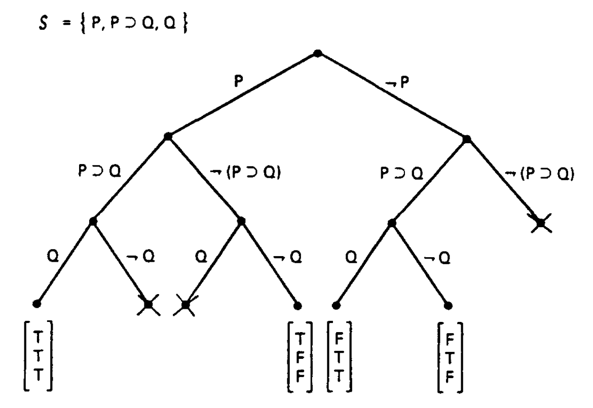
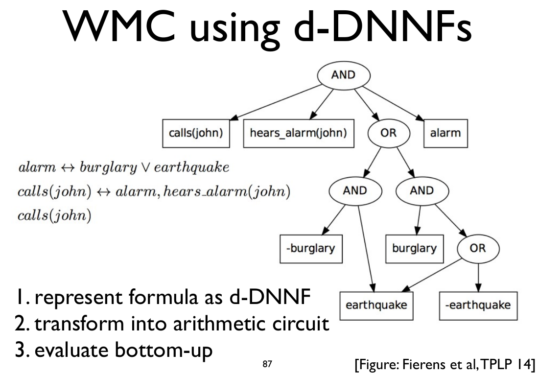
Inference

Weighted Model Counting: Compile logic formulae to a DAG then count possible worlds.

(De Raedt & Kimming, IJCAI 15 Tutorial)

Parameter Learning

Define the structure of logic rules:

%% Rules
t(_)::stress(X) :- person(X).
t(_)::influences(X,Y) :- person(X), person(Y).

smokes(X) :- stress(X).
smokes(X) :- friend(X,Y), influences(Y,X), smokes(Y).

%% Facts
person(1).   person(2).   person(3).   person(4).
friend(1,2). friend(4,2). friend(2,1). friend(2,4).
friend(3,2).

%% examples
evidence(smokes(2),false).
evidence(smokes(4),true).
evidence(influences(1,2),false).
evidence(influences(4,2),false).
evidence(influences(2,3),true).
evidence(stress(1),true).

Learned weights:

0.666666666666667::stress(X) :- person(X).
0.339210385615516::influences(X,Y) :- person(X), person(Y).

Heavy Reasoning / Light Learning

Cannot solve problems like this…

Heavy Reasoning / Light Learning

Very complex probabilistic logical inference
- Hard to use advanced symbolic optimisation techniques (Prolog, ASP, SAT, SMT, etc.)
- Usually use variational inference and other approximated methods
Symbolic representation
- Where do the symbols come from? (Russell, 2015)
Unnecessary independence assumptions
- Fuzzy operators, etc.
Hard to learn rule structure
- efficient inference only available with compiled rules
- Where do the rules come from?

A More Natural Way

The “head variants”

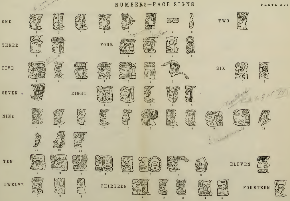
Mayan Calendar

Cracking the glyphs: They Must Be Consistent!

Explanation:

(1.18.5.4.0): the 275480 day from origin
(1 Ahau): the 40th day of that year
(13 Mac): in the 13 month of that year

Abductive Reasoning

Starts from incomplete observations, proceeds to the likeliest possible explanation for the set.

Data-driven / mostly noisy / low-level statistical perception
Knowledge-driven / mostly deterministic / high-level symbolic reasoning

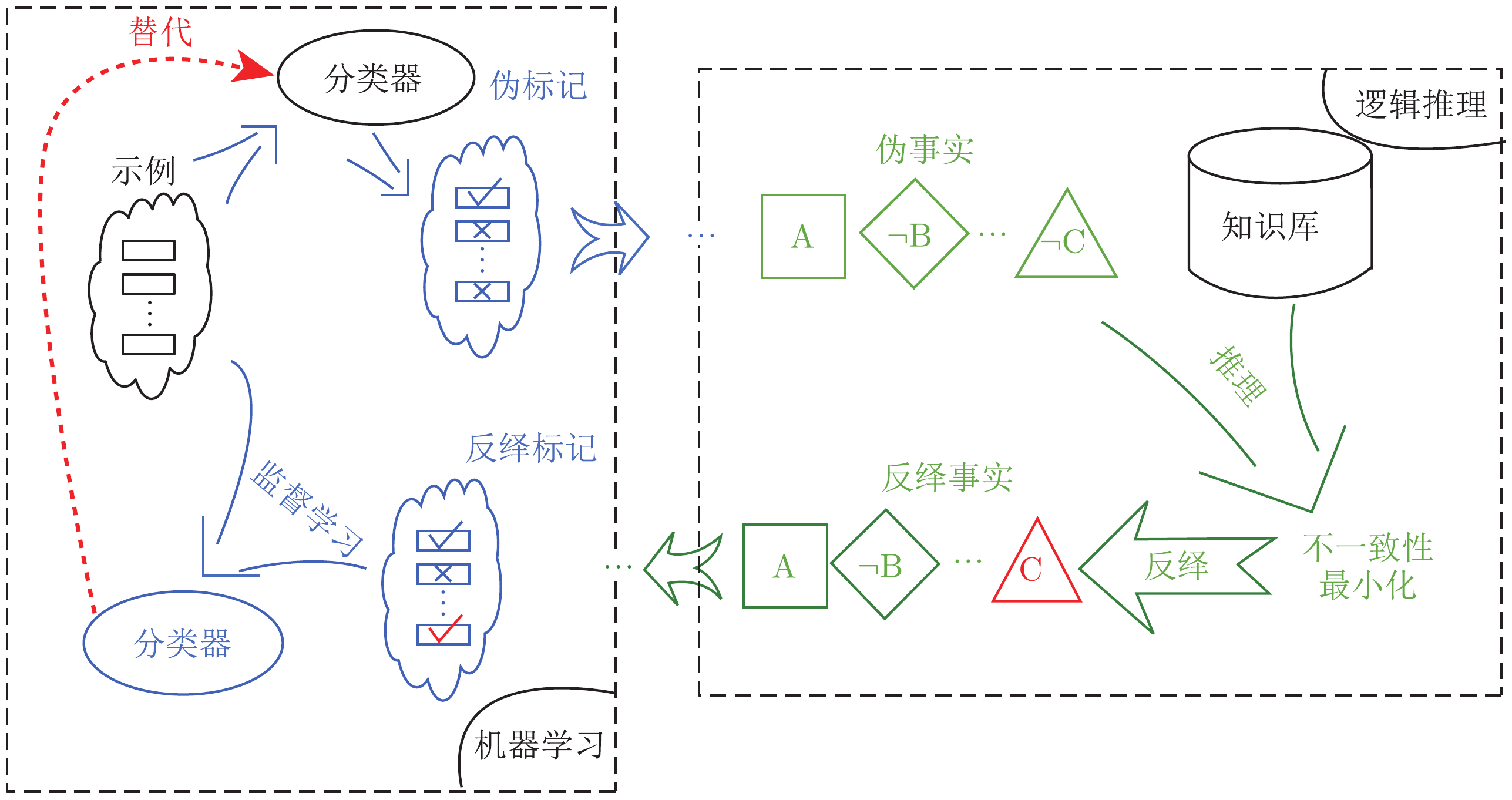
The Abductive Learning Framework (ABL)

Training examples: $⟨ x,y⟩ $.

Machine learning (e.g., neural net): \[ z=f(x;\theta)=\text{Sigmoid}(P_\theta(z|x))\]
- Learns a perception model mapping raw data ($x$) ⟶ logic facts (z);
Logical Reasoning (e.g., logic program): \[B\cup z\models y\]
- Deduction: infers the final output ($y$) based on $z$ and background knowledge ($B$);
- Abduction: infers pseudo label (revised facts) $z'$ to improve perception model $f(x;\theta)$;
- Induction: learns (first-order) logical theory $H$ such that $B\cup \color{#CC9393}{H}\cup z\models y$;
Optimisation:
- Maximises the consistency of $H\cup z$ and $f$ w.r.t. $\langle x, y\rangle$ and $B$.

Supervised Learning

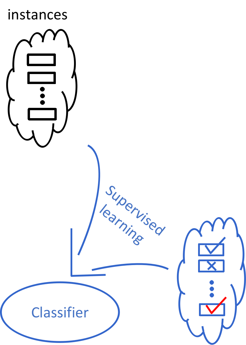
Abductive Learning

(Zhi-Hua Zhou. Abductive learning: Towards bridging machine learning and logical reasoning. In: Science China Information Sciences, 2019, 62: 076101.)

Handwritten Equation Decipherment

Task: Image sequence only with label of equation’s correctness

Untrained image classifier (CNN) $f:\mathbb{R}^d\mapsto\{0,1,+,=\}$
Unknown rules: e.g. 1+1=10, 1+0=1,…(add); 1+1=0, 0+1=1,…(xor).
Learn perception and reasoning jointly.

Implementation

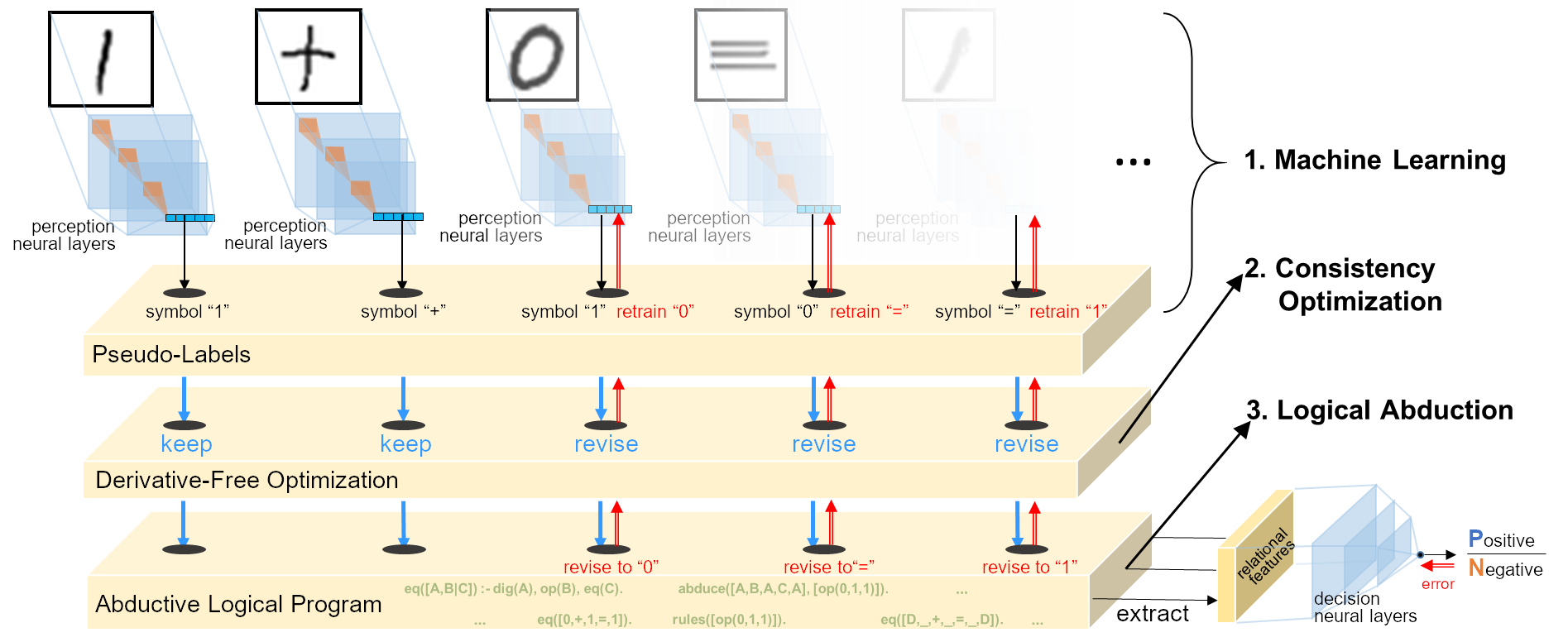
Optimise consistency by Heuristic Search

\begin{align} \max\limits_{\color{#CC9393}{\delta}}\quad&\sum_{(x,y)}\text{Con}({\color{#CC9393}{z'}}\cup H, B, y),\\ s.t.\quad& H\cup z'=\text{abduce}(B,z,{\color{#CC9393}{\delta}(z)}), \text{where }z=f(x;\theta_t),\\ &\text{Hamming}(z,z')\leq M \end{align}

Heuristic function for guessing the wrongly perceived symbols: \[\text{symbols to be revised}=\delta(z)\]
Abduce revised assignments of $\delta(z)$ that guarantee consistency: \[ B\cup H\cup \underbrace{\overbrace{z\backslash\delta(z)}^{\text{unchange}} \cup \overbrace{{\color{#CC9393}{r_\delta}}(z)}^{\text{revise}}}_{\text{pseudo-labels }z'} \models y \]

Experiment

Data: length 5-26 equations, each length 300 instances
- DBA: MNIST equations;
- RBA: Omniglot equations;
- Binary addition and exclusive-or.
Compared methods:
- ABL-all: Our approach with all training data
- ABL-short: Our approach with only length 7-10 equations;
- DNC: Memory-based DNN;
- Transformer: Attention-based DNN;
- BiLSTM: Seq-2-seq baseline;

Training Log

%%%%%%%%%%%%%% LENGTH:  7  to  8 %%%%%%%%%%%%%%
This is the CNN's current label:
[[1, 2, 0, 1, 0, 1, 2, 0], [1, 1, 0, 1, 0, 1, 3, 3], [1, 1, 0, 1, 0, 1, 0, 3], [2, 0, 2, 1, 0, 1, 2], [1, 1, 0, 0, 0, 1, 2], [1, 0, 1, 1, 0, 1, 3, 0], [1, 1, 0, 3, 0, 1, 1], [0, 0, 2, 1, 0, 1, 1], [1, 3, 0, 1, 0, 1, 1], [1, 0, 1, 1, 0, 1, 3, 3]]
****Consistent instance:
consistent examples: [6, 8, 9]
mapping: {0: '+', 1: 0, 2: '=', 3: 1}
Current model's output:
00+1+00 01+0+00 0+00+011
Abduced labels:
00+1=00 01+0=00 0+00=011
Consistent percentage: 0.3
****Learned Rules:
rules:  ['my_op([0],[0],[0,1])', 'my_op([1],[0],[0])', 'my_op([0],[1],[0])']

Train pool size is : 22

...
This is the CNN's current label:
[[1, 1, 0, 1, 2, 1, 3, 3], [1, 3, 0, 3, 2, 1, 3], [1, 0, 1, 1, 2, 1, 3, 3], [1, 1, 0, 1, 0, 1, 3, 3], [1, 0, 1, 1, 2, 1, 3, 3], [1, 1, 0, 1, 0, 1, 3, 3], [1, 0, 3, 3, 2, 1, 1], [1, 1, 0, 1, 2, 1, 3, 3], [1, 1, 0, 1, 2, 1, 3, 3], [3, 0, 1, 1, 2, 1, 1]]
****Consistent instance:
consistent examples: [0, 1, 2, 3, 4, 5, 6, 7, 8, 9]
mapping: {0: '+', 1: 0, 2: '=', 3: 1}
Current model's output:
00+0=011 01+1=01 0+00=011 00+0=011 0+00=011 00+0=011 0+01=00 00+0=011 00+0=011 1+00=00
Abduced labels:
00+0=011 01+1=01 0+00=011 00+0=011 0+00=011 00+0=011 0+01=00 00+0=011 00+0=011 1+00=00
Consistent percentage: 1.0
****Learned feature:
Rules:  ['my_op([1],[0],[0])', 'my_op([0],[1],[0])', 'my_op([1],[1],[1])', 'my_op([0],[0],[0,1])']

Train pool size is : 77

Performance

Test Acc. vs Eq. length

Abductive Knowledge Induction

Example: Accumulative Sum

A task from Neural arithmetic logic units (Trask et al., NeurIPS 2018).

Examples: Sequences of handwritten digit images ($x$) with their sums ($y$);
Task:
- Perception: An image recognition model $f: \text{Image}\mapsto \{0,1,\ldots,9\}$; \[z=f(x)=f([img_1, img_2, img_3])=[7,3,5]\]
- Reasoning: A program to calculate the output $y$.

:- Z = [7,3,5], Y = 15, prog(Z, Y).
% true.

How to write the prog?

Objective

\[ \underset{\theta}{\operatorname{arg max}}\sum_z \sum_H P(y,z,H|B,x,\theta) \]

$x$: noisy input
$y$: final output
$z$: unknown pseudo-labels (logic facts);
$\theta$: parameter of machine learning model;
$H$: missing logic rules (the prog).
$B$: background knowledge, e.g., primitive procedures

EM-based Learning

Expectation: Estimate the expectation of the symbolic hidden variables; \[\hat{H}\cup\hat{z}=\mathbb{E}_{(H,z)\sim P(H,z|B,x,y,\theta)} [H\cup z]\]
- Calculate the expectation by sampling: $P(H,z|B,x,y,\theta)\propto P(y,H,z|B,x,\theta)$ \[P(y,H,z|B,x,\theta)=\underbrace{P(y|B,H,z)}_{\text{logical abduction}} \cdot \overbrace{P_{\sigma^*}(H|B)}^{\text{Prior of program}} \cdot \underbrace{P(z|x,\theta)}_{\text{Prob. of Poss. Wrld.}}\]
Maximisation: Optimise the neural parameters to maximise the likelihood. \[\hat{\theta}=\underset{\theta}{\operatorname{arg max}}P(Z=\hat{z}|x,\theta)\]

Example: Abduction-Induction Learning

#= is a CLP(Z) predicate for representing arithmetic constraints:
- e.g., X+Y#=3, [X,Y] ins 0..9 will output X=0, Y=3; X=1, Y=2; ...

Experiments

Tasks: MNIST calculations
1. Accumulative sum/product;
2. Bogosort (permutation sort);
Compared methods and domain knowledge:

Domain Knowledge	End-to-end Models	$Meta_{Abd}$
Recurrence	LSTM & RNN	Prolog’s list operations
Arithmetic functions	`NAC` & `NALU` (Trask et al., 2018)	Predicates `add`, `mult` and `eq`
Permutation	Permutation matrix $P_{sort}$ (Grover et al., 2019)	Prolog’s `permutation`
Sorting	`sort` operator (Grover et al., 2019)	Predicate `s` (learned as sub-task)

Accumulative Sum/Product

Learned Programs:

%% Accumulative Sum
f(A,B):-add(A,C), f(C,B).
f(A,B):-eq(A,B).

%% Accumulative Product
f(A,B):-mult(A,C), f(C,B).
f(A,B):-eq(A,B).

Bogosort

Learned Programs:

% Sub-task: Sorted
s(A):-s_1(A,B),s(B).
s(A):-tail(A,B),empty(B).
s_1(A,B):-nn_pred(A),tail(A,B).

%% Bogosort by reusing s/1
f(A,B):-permute(A,B,C),s(C).

The subtask sorted/1 uses the subset of sorted MNIST sequences in training data as example.

Program Induction: Abductive vs Non-Abductive

$z\rightarrow H$: Sample $z$ according to $P_\theta(z|x)$ and then call conventional MIL to learn a consistent $H$;
$H\rightarrow z$: Combining abduction with induction using $Meta_{abd}$.

Conclusion

Conclusions

Summary

Full-featured logic programs:
- Handles heavy-reasoning problems & has better generalisation
- Exploits symbolic domain knowledge
- Learns recursive programs and invents predicates
Requires much less training data
Flexible framework with switchable parts:
- Possible to plug in many symbolic AI approaches;

Future work

Improving the optimisation efficiency;
New symbol discovery instead of defining every primitive symbols before training;

Thanks!

References:

Combining Machine Learning and Logical Reasoning

Two AI Paradigms

Data-Driven AI

Knowledge-Driven AI

Example: Learning Quick Sort

Combining Subsymbolic and Symbolic AI

System 1 vs System 2

Boolean Algebra

Many-Valued Logic

“Next-Gen” AI

Route 1:Statistical / Neural Relational Models

Knowledge Base Model Construction

KBANN (Towell & Shavlik, 1994)

Markov Logic (Richards & Domingos, 2006)

Modern Neuro-Symbolic Methods

Graph Neural Nets

Heavy Learning / Light Reasoning

Heavy Learning / Light Reasoning

Route 2: Probabilistic Logic

Distribution Semantics (Nilsson, 1986; Sato, 1995)

Probabilistic Logic Programs

Inference

Parameter Learning

Heavy Reasoning / Light Learning

Heavy Reasoning / Light Learning

A More Natural Way

The “head variants”

Mayan Calendar

Cracking the glyphs: They Must Be Consistent!

Abductive Reasoning

The Abductive Learning Framework (ABL)

Supervised Learning

Abductive Learning

Handwritten Equation Decipherment

Implementation

Optimise consistency by Heuristic Search

Experiment

Training Log

Performance

Abductive Knowledge Induction

Example: Accumulative Sum

Objective

EM-based Learning

Example: Abduction-Induction Learning

Experiments

Accumulative Sum/Product

Bogosort

Program Induction: Abductive vs Non-Abductive

Conclusion

Conclusions

Thanks!

Route 1:
Statistical / Neural Relational Models

Route 2:
Probabilistic Logic

References:

- W.-Z. Dai, S. H. Muggleton. Abductive Knowledge Induction From Raw Data, arXiv, 2010.03514, 2020.
- Y.-X. Huang, W.-Z. Dai, J. Yang, L.-W. Cai, S. Cheng, R. Huang, Y.-F. Li and Z.-H. Zhou, Semi-Supervised Abductive Learning and Its Application to Theft Judicial Sentencing, In: Proceedings of 20th IEEE International Conference on Data Mining (ICDM’20). Sorrento, Italy, 2020.
- W.-Z. Dai, Q.-L. Xu, Y. Yu, and Z.-H. Zhou. Bridging machine learning and logical reasoning by abductive learning. In: Advances in Neural Information Processing Systems 32 (NeurIPS’19). Vancouver, Canada, 2019.
- Z.-H. Zhou. Abductive learning: Towards bridging machine learning and logical reasoning. Science China Information Sciences, 2019, vol.62, 076101.